You are here: Autotuning
Autotuning
The tuning functions adjust the manufacturer’s default values to the load conditions in order to keep tracking errors to a minimum. You must optimize the control loops for highly dynamic or high-precision applications manually.
Autotuning can be initiated multiple times, because the results are cumulated (Initial Quality).
|
|

|
Automatic Start!
|
During the tuning functions, the servo amplifier is enabled and the load can move. Risk of injury. To avoid dangerous situations, take note of the following information:
- For vertical axes: Move the load manually to bottom dead center and set the direction of motion to “negative only” or “positive only” (depending on the application) before you begin the test or tuning functions.
- For feedback without commutation: Perform a Wake and Shake first.
- Release the parking brake.
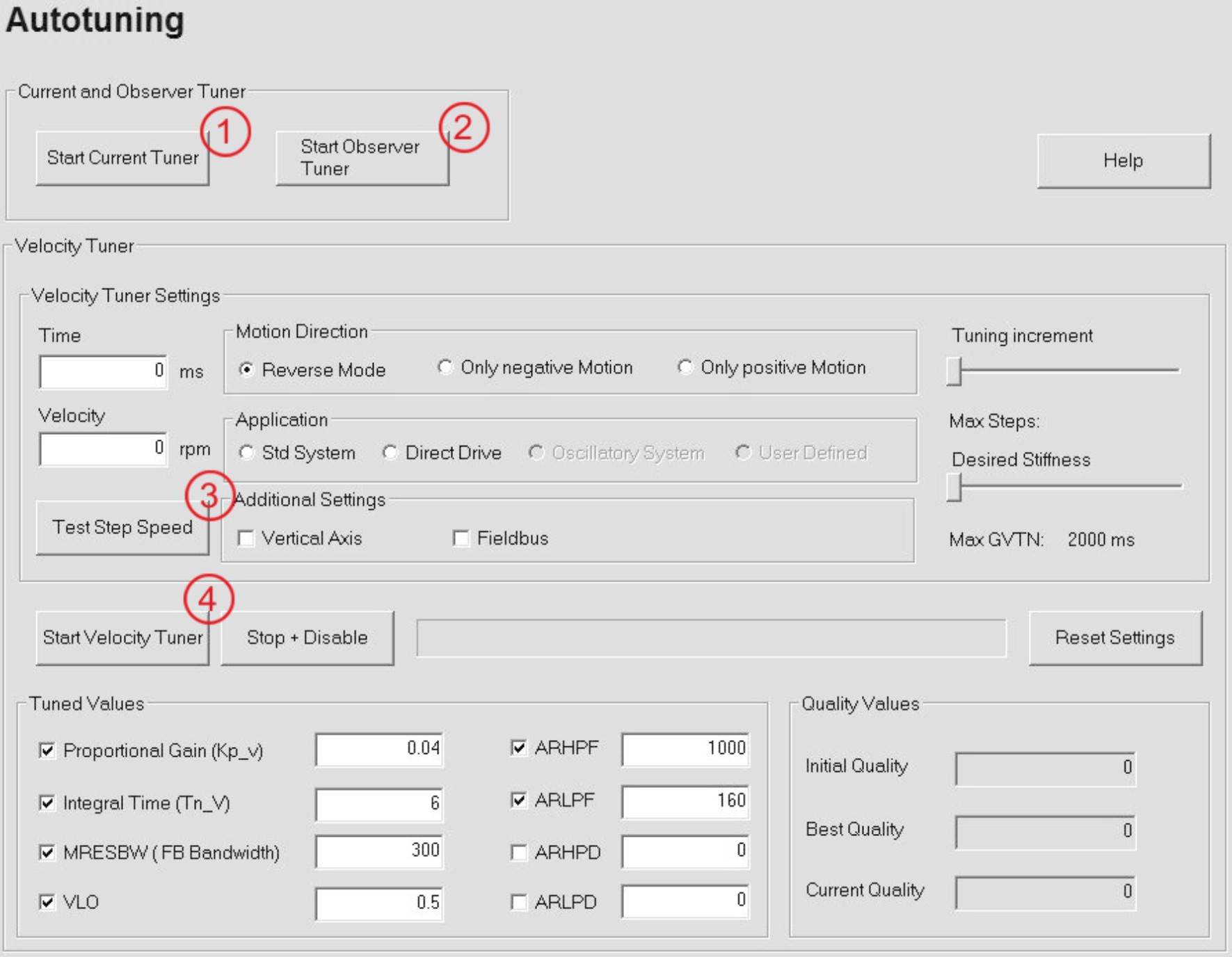
- Perform autotuning in 4 steps (see screenshot). All functions enable the output stage and result in motor axis motions:
1- Current Tuning
2 - Observer Tuning
3 - Test Step Speed for Autotuning
4 - Autotuning
|
The setup software automatically checks whether autotuning is implemented in the firmware and activates the functions. If the firmware does not support autotuning, the relevant page is still shown although the control elements will be deactivated.
Prerequisite:
- The motor and feedback settings must be correct. In the case of feedback systems without commutation, Wake and Shake must have been performed.
- The load must be connected.
- The drive parking brake must not be on.
Current and Observer Tuning
|
Start Current Tuner
|
This button starts the tuning function for the current controller. For this to occur, OPMODE must be set to 2.
|
| Start Observer Tuner
|
This button starts an optimization function for the VLO parameter.
VLO is a parameter of the Luenberger speed observer. Reducing VLO excessively may compromise the stability of the speed control loop.
|
Test Step Speed
The axis is now preset to the extent that an initial motion test can take place. To perform this, switch to the „Oszilloscope“ page.
Under „Motion Service“, you can select the operating function and enter the motion parameters.
|
Horizontal/Rotary Axes:
|
Move the axis to the central position. Use the reverse operation function for an initial test run. Set the parameters to safe values.
ATTENTION: Stop the motion manually (Stop button or F11).
|
| Vertical Axes:
|
Move the axis to bottom dead center. Use the Select Speed (Velocity) function for an initial test run. Set the parameters to safe values.
ATTENTION: Stop the motion manually (Stop button or F11).
|
If the axis does not move with the default speed controller parameters, you may increase the proportional amplification “GV” until a motion can be observed. During service operation, you can change the parameters on the Oscilloscope page, under „Tuning“.
During test mode, start a Recording and save the image as a reference recording so that you can compare and evaluate the results after autotuning. For this purpose, save the recordings in a file.
Now you can proceed with autotuning. Go back to the Autotuning page.
Velocity Loop Tuning
TIP: The slew rate of the jumps is defined by ACC and DEC. To ensure reliable results, the highest possible slew rate should be selected (observing the limitations of the machinery).
| Time |
In this field, enter the time in ms during which the axis should move at the speed specified below. This value is used in both positive and negative directions, provided that the direction of motion is not restricted. High moments of inertia require more time.
|
| Velocity
|
In this field, enter the speed at which the axis should move. The unit of speed is dependent upon the settings that have been made. The speed is used in both positive and negative directions, provided that the direction of motion is not restricted.
|
| Motion Direction
|
Here you can specify whether the axis may move in both directions or just in one particular direction.
Do not use reverse mode for vertical axes!
Please note that the direction of rotation is dependent upon the parameter „“, which is used to define the direction.
|
| Application
|
The filter strategy is adapted to the relevant target application using the application selection. If filter parameters are selected manually, the application is automatically set to user-defined.
Def. System: PIDT2 filter (frequencies initially set to def.)
Direct Drive: All filters deactivated
Oscillating System: BIQUAD filter (frequencies and attenuation are initially set to def.). Not currently implemented!
User-defined: Only manually selected filters are tuned
|
| Additional Setting
|
Fieldbus: Select this check box if the position/speed specifications of the target application are set using a fieldbus. If this is the case, a modified tuning strategy is used.
Vertical Axis: When dealing with a vertical axis or an axis which is subjected to a constant level of force (such as a spring), this function must be activated. With this kind of axis, the integral component (GVTN) is not deactivated during the tuning process.
|
| Tuning increment
|
You can use this slide control to limit the maximum step width. This enables sensitive superstructures to be protected, as only small step widths are used to modify the parameters. However, reducing the step width of the tuning algorithm increases the algorithm run time.
|
|
Desired Stiffness
|
The lower the integral component (GVTN) setting, the more rigid the axis.
The slider sets the value range for GVTN :
Left: 0 ≤ GVTN ≤ 2000ms
Right: 0 ≤ GVTN ≤ 10ms
|
|
Tuned Variable
|
For experienced users: You can exclude individual parameters from the tuning process or tune particular parameters only. This also applies to the filter parameters. If the filter parameters are selected manually, the target application is automatically set to user-defined.
|
ASCII Parameter
|
Description
|
|
GV
|
Proportional gain
|
|
MRESBW
|
Feedback Bandwidth
|
|
VLO
|
Observer feed forward
|
|
GVTN
|
Integral Time
|
|
ARLPF
|
Filter low pass frequency
|
|
ARHPF
|
Filter high pass frequency
|
|
ARLPD
|
Filter low pass damping
|
|
ARHPD
|
Filter high pass damping
|
|
| Start Velocity Tuner
|
Click the button to start the autotuning routine. The cursor is shown as “busy” during the tuning process and a progress bar displays the tuning status. During the tuning process, it is possible to observe the I²T utilization of the servo amplifier on the Monitor page, for example.
Tuning is complete once the progress bar reaches 100% and the Start Auto-Tuning button is reactivated. You can then restart the tuning process using different parameters and settings, or compare the results with the reference measurements by performing a new oscilloscope recording with the same motion parameters.
|
| Stop + Disable |
Click the button to stop the autotuning routine. The servo amplifier is disabled and the current values are located in the volatile memory. Exiting the window also stops the autotuning routine.
|
| Initial Quality
|
Condition at the start of the autotuning function
|
| Current Quality
|
Results achieved at the present time
|
| Best Quality
|
Best results achieved to date
|
Autotuning lowers GV by around 20% below the determined maximum value in order to provide resilient settings. With highly dynamic applications, GV can be raised by 20% again.
Save the determined values in the EEPROM.
|
|
Copyright © 2020
|
|

|


